The rapid adoption of Retrieval-Augmented Generation (RAG) and semantic search has forced engineering teams to make a critical architectural decision: Should you store and query your vector embeddings in your existing relational database using an extension like pgvector, or should you spin up a specialized vector database like Qdrant, Milvus, or Pinecone?
While the allure of specialized databases is strong—promising sub-millisecond latencies and billion-scale capacity—the operational complexity of introducing a new database into your stack is often underestimated. Conversely, treating Postgres as a one-size-fits-all solution can lead to severe memory bottlenecks and degraded performance if your vector workload outgrows your hardware resources.
This article breaks down the real-world cost, performance, and operational tradeoffs between Postgres with pgvector and specialized vector databases, helping you make an informed decision for your production stack.
The Mechanics of Vector Search
Vector search is fundamentally different from traditional relational querying. Instead of matching exact values, range boundaries, or text patterns, vector search calculates the mathematical distance between high-dimensional vectors (embeddings) generated by machine learning models. These embeddings represent the semantic meaning of text, images, or audio.
When building modern AI applications, developers often need to connect their Large Language Models (LLMs) to enterprise databases. For a deeper dive into standardizing these connections, see our guide on the Model Context Protocol (MCP) Explained: How to Connect LLMs to Real-World Data (With Python Tutorial).
To perform semantic search, the database must calculate the distance between a query vector and millions of stored vectors. Common distance metrics include:
- Cosine Distance: Measures the angle between two vectors, ignoring magnitude. Ideal for text embeddings where document length varies.
- L2 (Euclidean) Distance: Measures the straight-line distance between two points in Euclidean space. Useful when vector magnitude is important.
- Inner Product (Dot Product): Calculates the projection of one vector onto another. If vectors are normalized (magnitude of 1), this is mathematically equivalent to cosine distance but significantly faster to compute.
Doing this naively requires a full table scan (exact nearest neighbor search), which is computationally prohibitive at scale. To solve this, databases use Approximate Nearest Neighbor (ANN) indexes to trade a small amount of accuracy (recall) for massive speedups.
Deep Dive into pgvector: Vector Search Inside the Relational Engine
pgvector is an open-source extension for PostgreSQL that introduces a native vector data type, along with distance operators and indexing mechanisms. It allows you to store embeddings directly alongside your relational data, maintaining strict ACID compliance and leveraging your existing Postgres infrastructure.
Indexing Strategies: IVFFlat vs. HNSW
pgvector supports two primary index types for accelerating vector queries:
- IVFFlat (Inverted File with Flat Compression): This index divides vectors into lists (clusters) using k-means clustering. When querying, it only searches the closest clusters.
- Pros: Fast build times, low memory footprint.
- Cons: Lower recall (accuracy) and slower query performance compared to HNSW as the dataset grows.
- HNSW (Hierarchical Navigable Small World): This index builds a multi-layer graph structure where nodes represent vectors and edges represent proximity.
- Pros: Exceptional query latency and high recall.
- Cons: Extremely slow index build times and high memory consumption, as the entire graph must reside in RAM for optimal performance.
Code Example: Implementing pgvector
Setting up pgvector is straightforward. For Java developers looking to interface with Postgres, choosing the right abstraction layer is critical. Read our comparison of JPA vs Hibernate vs JDBC: What Is the Difference? to optimize your database access patterns. Below is a raw SQL example demonstrating how to configure and query vectors in Postgres:
-- Enable the pgvector extension
CREATE EXTENSION IF NOT EXISTS vector;

-- Create a table storing document chunks and their 1536-dimensional embeddings
CREATE TABLE document_embeddings (
    id BIGSERIAL PRIMARY KEY,
    content TEXT NOT NULL,
    metadata JSONB,
    embedding vector(1536)
);

-- Insert a record with a vector
INSERT INTO document_embeddings (content, embedding)
VALUES ('Postgres is highly extensible.', '[0.012, -0.023, 0.456, ...]');

-- Create an HNSW index for Cosine Distance
CREATE INDEX ON document_embeddings
USING hnsw (embedding vector_cosine_ops);

-- Query the 5 most semantically similar documents
SELECT id, content, 1 - (embedding <=> '[0.015, -0.020, 0.440, ...]') AS similarity
FROM document_embeddings
ORDER BY embedding <=> '[0.015, -0.020, 0.440, ...]'
LIMIT 5;
In this query, the <=> operator represents cosine distance. Subtracting it from 1 yields the cosine similarity score.
Specialized Vector Databases: Built for High-Dimensional Scale
Specialized vector databases (such as Qdrant, Milvus, and Pinecone) are designed from the ground up for vector operations. They do not treat vectors as an extension of a relational table; instead, they treat the vector index as the primary data structure.
These databases utilize custom-built execution engines optimized for SIMD (Single Instruction, Multiple Data) hardware acceleration, allowing them to perform vector math directly on CPU registers or GPUs. They also implement advanced quantization techniques (like Product Quantization or Scalar Quantization) to compress vectors, reducing the memory footprint by up to 95% at the cost of a minor loss in precision.
The Architectural Cost of the “Dual-Write” Problem
While specialized databases offer blistering performance, they introduce a major architectural headache: the dual-write problem.
In a specialized architecture, your metadata (users, permissions, document text) lives in your primary relational database (e.g., Postgres), while your embeddings live in the vector database. When a user updates a document, your application must write to both databases. This introduces several risks:
- Eventual Consistency: If the write to the vector database fails or is delayed, your search index becomes out of sync with your primary database.
- Complex Transactions: You lose ACID guarantees. Rolling back a transaction across two physically distinct databases requires complex distributed transaction patterns (like the Saga pattern).
- Data Redundancy: To perform filtered vector searches (e.g., “find vectors matching query X but only for tenant Y”), you must duplicate metadata into the vector database so it can perform pre-filtering or post-filtering.
Performance, Memory, and Cost Tradeoffs
To understand the real tradeoffs, we must look at how these systems handle resources under load.
The Memory Bottleneck: RAM vs. Disk
For HNSW indexes, both pgvector and specialized databases require the index to live in RAM. If your index exceeds available RAM, the operating system will swap to disk, causing query latencies to spike from milliseconds to seconds.
Let’s calculate the memory required for a dataset of 10 million vectors with 1536 dimensions (the standard for OpenAI’s text-embedding-3-small model) using an HNSW index:
- Raw Vector Data: $$10,000,000 \times 1536 \times 4 \text{ bytes (float32)} = 61,440,000,000 \text{ bytes} \approx 61.44 \text{ GB}$$
- HNSW Graph Overhead: HNSW requires additional memory to store the graph edges. A typical configuration ($M=16$, $ef_construction=64$) adds roughly 20-30% overhead. $$\text{Total Memory Required} \approx 75 \text{ to } 80 \text{ GB}$$
In Postgres, this entire 80 GB index must fit into the shared buffers or OS cache. Because Postgres is also handling relational queries, transactions, and joins, you will need a database instance with at least 128 GB of RAM to prevent resource starvation. Understanding these hardware fundamentals (RAM, CPU, storage IOPS) is critical for systems design; for a solid foundational review, see The Ultimate CompTIA Tech+ Cheatsheet: Mastering the Fundamentals of IT.
If you are orchestrating these databases on cloud platforms like Microsoft Azure, understanding cloud resource provisioning is essential. Check out our AZ-900 Cheatsheet: The Complete Azure Fundamentals Study Guide for a comprehensive overview of cloud infrastructure.
Specialized vector databases handle this more efficiently. They can use scalar quantization to compress the 32-bit floating-point numbers into 8-bit integers, reducing the raw vector memory footprint from 61.44 GB to just 15.36 GB. This allows you to serve the same 10 million vectors on a much smaller, cheaper instance.
Latency and Throughput at Scale
Performance comparisons are meaningful only when both systems use the same embeddings, recall target, filter selectivity, concurrency, hardware class, index build state, and measurement window. Treat latency and throughput as workload-specific observations rather than properties of a product category, and record the operational cost required to obtain each result.
Filtering Strategies: The Hidden Killer of Specialized DBs
In real-world applications, you rarely perform a pure vector search. Instead, you perform a filtered vector search: “Find the most similar documents created by user X in the last 30 days.”
There are three ways to handle this:
- Post-filtering: The database performs a vector search first, gets the top 100 results, and then filters out those that do not match the metadata criteria. If only 2 of those 100 match the criteria, you return only 2 results instead of the requested limit.
- Pre-filtering: The database filters the metadata first, then performs a vector search on the remaining documents. If the filter is highly restrictive (e.g., matching only 10 documents out of millions), building an HNSW graph on the fly for those 10 documents is incredibly slow.
- Single-stage (Iterative) Filtering: The database traverses the HNSW graph and evaluates the metadata filter at each step of the graph traversal. This is the gold standard.
Postgres handles single-stage filtering natively and elegantly because its query planner can combine relational indexes (B-Trees) with vector indexes. Specialized vector databases must implement complex custom indexing engines to achieve similar results, which often require duplicating your relational schema inside the vector database.
Architectural Comparison
The table below summarizes the core differences between Postgres with pgvector and specialized vector databases:
| Feature | Postgres with pgvector | Specialized Vector DB (e.g., Qdrant, Milvus) | SaaS Vector DB (e.g., Pinecone) |
|---|---|---|---|
| Primary Index Types | HNSW, IVFFlat | HNSW, DiskANN, IVF-PQ | Proprietary (Optimized HNSW/Graph) |
| Max Recommended Scale | ~10M - 50M vectors | Billions (Distributed) | Billions (Serverless) |
| Query Latency (1M vectors) | Low (2-10ms) | Ultra-low (1-5ms) | Low-to-Medium (5-15ms via API) |
| Relational Joins | Native, instant | Impossible (Requires application-level join) | Impossible |
| ACID Compliance | Yes (Full) | No (Eventual consistency) | No (Eventual consistency) |
| Operational Complexity | Zero (Existing Postgres instance) | Medium (Requires managing a new cluster) | Low (Fully managed API) |
| Cost Model | Resource-based (Compute/RAM) | Resource-based (Compute/RAM) | Usage-based (Read/Write units & storage) |
Visualizing the Architectures
To better understand how these systems differ in practice, let’s look at the architectural flow of a query in both setups.
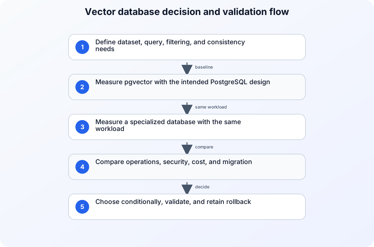
The unified approach can simplify application logic by keeping relational data and embeddings within one database boundary. A split architecture introduces a second datastore and therefore requires explicit ownership for synchronization, access control, failure recovery, and reconciliation when one write succeeds and the other fails.
When scaling these systems in production, organizations must decide whether to manage this infrastructure themselves or rely on managed cloud services. For instance, running enterprise AI workloads at scale often involves deploying models alongside highly optimized database layers. This is similar to how enterprises leverage managed environments like Claude on Google Cloud to handle global compliance and low-latency inference.
Furthermore, if you choose to deploy specialized vector databases on Kubernetes, the operational overhead increases significantly. Operators must monitor custom resources and pod lifecycles closely, often using specialized tools like Kubeflow and Headlamp plugins to observe ML workloads at the cluster level. For distributed coordination, these specialized databases often rely on consensus engines like etcd, which requires careful tuning of range streams and storage backends to maintain cluster state under high write loads.
Decision Framework: When to Choose Which
To make the right choice, evaluate your workload against the following criteria:
Choose Postgres with pgvector if:
- Your dataset is under 10 million vectors: At this scale, a moderately sized Postgres instance can easily hold the HNSW index in memory.
- You require strict ACID compliance: If your vector search results must immediately reflect updates made to your relational data (e.g., hiding a document immediately after a user deletes it), Postgres is the only sensible choice.
- You rely heavily on metadata filtering: If your queries look like “find similar documents where user_id = 42 AND status = ‘active’”, Postgres’s query planner will outperform specialized databases by executing single-stage filtering natively.
- You want to minimize operational overhead: Keeping your stack simple prevents “architectural bloat” and reduces the number of moving parts your team has to monitor and maintain.
Choose a Specialized Vector Database if:
- Your dataset exceeds 50 million vectors: At this scale, the memory requirements for HNSW will overwhelm a single Postgres instance, requiring a distributed vector database that can shard indexes across multiple nodes.
- You require ultra-high write throughput: Postgres indexes (especially HNSW) are slow to build and update. If you are constantly streaming and indexing millions of new vectors per hour, a specialized database with asynchronous index building is required.
- You need advanced quantization: If you want to run large vector datasets on a budget, specialized databases that support Product Quantization (PQ) can drastically reduce your RAM costs.
Conclusion
For the vast majority of engineering teams, Postgres with pgvector is the correct starting point. It eliminates the dual-write problem, maintains strict transactional guarantees, and leverages your existing operational knowledge. Only when your dataset approaches tens of millions of vectors, or when your write throughput bottlenecks your relational engine, should you take on the operational complexity of a specialized vector database.